Astronomical Imaging and FITS#
Gather round, for I shall tell a tale old as time. Long, long ago, astronomers gazed at the heavens, and with naught but their eyes, recorded the positions of the stars they saw there. Then, with the telescope, long, heavy contraptions which reached for the skies like an outstretched arm, (thanks, f/20 focal lengths) they gazed through eyepieces in freezing domes, falling, on occasion, to their deaths from cages suspended at prime foci.
Next came glass – emulsion plates – which upon extended exposure revealed upon their ghostly frames the splotches of stars and soon, galaxies and nebulae. Many a grad student, of course, spent their nights twiddling thumbs over micrometer dials to keep these stars in place. Manual guiding… this story teller shudders to imagine it. And yet, even then, with permanent record, no measure could be made that weren’t ‘tween the eyes of an observer, peering at the glass through magnifying eyepiece, assigning grades of brightness and, amazingly, pretty much nailing the spectral classification of stars by their absorption features.
And after this painstaking work, came the earliest CCDs, fractured by detector failures, riddled with readout noise, consumed by cosmic ray hits, laid low by low quantum efficiencies.
Now… we use Python.
What’s in an image#
Astronomical images differ from standard images taken with a phone or DSLR camera primarily in that they both use older CCD technology and are typically “black and white”, recording only intensity of light and not color.
Knowledge about color instead comes from the placement of filters in front of the detectors which have a certain bandpass, allowing through light within a certain wavelength range and blocking light outside it.
Thus, we only ever get one color at a time, unless the telescope splits incoming light by color using, for example, a dichroic, and then sends the two streams to two detectors with different filters simultaneously.
This means that in some sense, single-band (i.e., one narrow-ish wavelength range) images are simple programmatically: They are 2D arrays in which each pixel (position in array) contains a single number: counts (in some units).
Usually, these units are counts in ADU (analog-to-digital units), which are roughly related to the actual counts of photons hitting the detector, via properties such as the gain of the system.
Generally, we are not concerned with the exact units/gain/etc., because we back out the flux in photons (or energy, rather) via empirical calibrations with objects in the sky of known flux. Sometimes, we are given images that have already been flux calibrated, in which case measurements of, say, counts in an aperture are real flux units.
Image Handling with Astropy#
Lastly, we need to know how to work with astronomical images in Python. As “simple” 2D arrays, simply opening and plotting an image is easy. But keeping track of, say, the celestial coordinates associated with a pointing on the sky, is not.
Luckily, the open-source astropy library has many tools that facilitate the streamlined handling of astronomical imaging.
Opening the Image#
Opening images using astropy is made easy using the fits file handler. We’ll use a context manager to read in an image:
from astropy.io import fits

with fits.open('antenna_Rband.fits') as hdu:
    header = hdu[0].header
    image = hdu[0].data
Note
A context manager is a useful tool for properly managing external resources in your programs. In this case, the external resource is a FITS file. When opening almost any file directly in Python, we also want to close our connection to that file once we have pulled out the data we need. A context manager, using python’s with above, will automatically close our fits file once extracting the header and image.
We can confirm we’ve loaded a 2D array:
image
array([[ 4.8691406,  5.432617 ,  5.713867 , ..., 11.48584  , 11.48584  ,
        11.48584  ],
       [ 5.573242 ,  5.713867 ,  5.291504 , ..., 11.48584  , 11.48584  ,
        11.48584  ],
       [ 6.4179688,  5.573242 ,  5.573242 , ..., 11.48584  , 11.48584  ,
        11.48584  ],
       ...,
       [11.48584  , 11.48584  , 11.48584  , ...,  6.2768555,  5.432617 ,
         5.9956055],
       [11.48584  , 11.48584  , 11.48584  , ...,  5.291504 ,  5.432617 ,
         5.573242 ],
       [11.48584  , 11.48584  , 11.48584  , ...,  5.291504 ,  4.8691406,
         3.4614258]], dtype=float32)
We can make a basic plot showing it:
fig, ax = plt.subplots(figsize=(6,6))
ax.imshow(image)
<matplotlib.image.AxesImage at 0x7fcfd9379bb0>
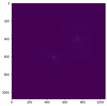
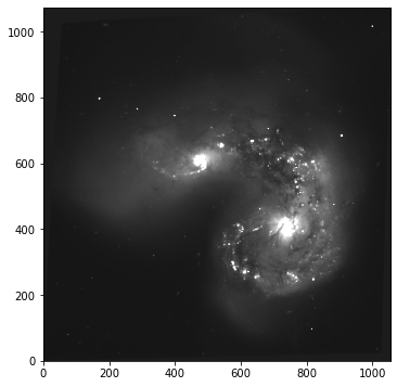
That may not have looked like much, but it did at least confirm we have a 2D image. Let’s tweak some settings.
import numpy as np
fig, ax = plt.subplots(figsize=(6,6))
m = np.mean(image)
s = np.std(image)
ax.imshow(image,origin='lower',vmin=m-s,vmax=m+5*s,cmap='gray');
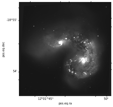
Next, we need to plot with our \(x\) and \(y\) axes representing sky coordinate (RA/DEC) rather than pixel position. For this, we’ll need to use astropy’s World Coordinate System module. There are several defined coordinate systems on the sky, but for this class, we’ll primarily be using RA and DEC. (i.e., equitorial coordinates measured in hour angles and degrees).
from astropy.wcs import WCS

wcs_im = WCS(header)
INFO:
                Inconsistent SIP distortion information is present in the FITS header and the WCS object:
                SIP coefficients were detected, but CTYPE is missing a "-SIP" suffix.
                astropy.wcs is using the SIP distortion coefficients,
                therefore the coordinates calculated here might be incorrect.

                If you do not want to apply the SIP distortion coefficients,
                please remove the SIP coefficients from the FITS header or the
                WCS object.  As an example, if the image is already distortion-corrected
                (e.g., drizzled) then distortion components should not apply and the SIP
                coefficients should be removed.

                While the SIP distortion coefficients are being applied here, if that was indeed the intent,
                for consistency please append "-SIP" to the CTYPE in the FITS header or the WCS object.

                 [astropy.wcs.wcs]
WARNING: FITSFixedWarning: 'datfix' made the change 'Set MJD-OBS to 53207.000000 from DATE-OBS'. [astropy.wcs.wcs]
The wcs for a given image is constructed from the image header, where some information about the pixel scale and image pointing are stored. Notice here we got a warning. This happens sometimes with HST images that are mosaics of pointings that have already been drizzled (an image alignment/combination process). We need to remove the mentioned coefficients.
The following will be provided for lab:
def strip_SIP(header):
    A_prefixes = [i for i in header.keys() if i.startswith('A_')]
    B_prefixes = [i for i in header.keys() if i.startswith('B_')]
    for a,b in zip(A_prefixes,B_prefixes):
        del header[a]
        del header[b]
    return header
header_fixed = strip_SIP(header)
wcs = WCS(header_fixed)
We are now ready to plot our image in celestial coordinates. Our game plan is to use matplotlib’s projection. You may be familiar with this as the way to make an axis, e.g., in polar coordinates. Astropy WCS objects can be treated as projections in matplotlib. Below I show two ways to initialize an axis with our new wcs projection.
fig, ax = plt.subplots(figsize=(6,6),subplot_kw={'projection':wcs})
fig = plt.figure(figsize=(6,6))
ax = fig.add_subplot(projection=wcs)

The two methods work equally well. The former is slightly preferred, as it makes it easy to make multiple panels with a wcs projection.
Now, all we have to do, is plop our image into it:
fig, ax = plt.subplots(figsize=(6,6),subplot_kw={'projection':wcs})
ax.imshow(image,origin='lower',vmin=m-s,vmax=m+5*s,cmap='gray');
ax
<WCSAxesSubplot:xlabel='pos.eq.ra', ylabel='pos.eq.dec'>
Lab Preview#
In this lab, you’ll be working with the same image of the Antenna galaxy, in several bands. In addition to the basic reading in and use of header/wcs, you’ll be learning about SkyCoord, the astropy handler for coordinates, and units which is a module we’ll be discussing throughout class. You’ll use Cutout2D to make zoom in plots of the image while retaining coordinate information. And you’ll use the photutils package and sep to find sources and perform some aperture photometry.
Lab: Astronomical Images#
Astronomical images are one of the basic building blocks of astronomical research. While we now obtain data in myriad ways, from gravitational waves to neutrinos, from spectra to polarimetry, the basic tenant of astronomy (and it’s most recongizable public impact) is the images we make of the sky.
That is why the first science topic we’ll be tackling is imaging. And along the way, we’ll learn how astropy makes our lives so much easier when dealing with images, and how to use robust functions to perform the analyses one might want to carry out on images (after we’re done admiring their beauty).
Many of you are probably familiar with the FITS standard. It stands for Flexible Image Transport System, and for all intents and purposes, it acts as a container (much like a zip file). Within it, one can store several kinds of information: images (2d arrays of values), as the name implies, headers (dictionary like objects with metadata), and sometimes tabular data as well. A FITS file can contain any number of extensions, which just refer to “slots” where stuff is stored. Every “slot” has a header attribute and a data attribute. Thus, you could store a hundred astronomical images in 1 file, each with a different extension and a different header describing the image in that slot.
Tip
Contextual clues are important when dealing with FITS files. Files that are explicitly single images almost always have the image stored in the 0th extension, while files that are explicitly table data tend to have the table stored in the 1st extension (with the 0th empty).
The FITS standard is pretty old, and may be retired soon, but almost all ground based telescopes still use it for their native image output, so it behooves us to know how to get image data out of FITS files.
Exercise 1: Loading a FITS File
Write a function which takes as its argument a string filepath to a FITS file, and should have an optional argument to set the extension (default 0). It should then load the given extension of that fits file using a context manager, and return a tuple containing the header and data of that extension.
The function should have documentation that describes the inputs and outputs.
Then use your function to read in the antennae R-band image.
# Your Code Here
Exercise 2.1: Plotting
Next, we need to plot the image data. There are several operations that we almost always perform when plotting astronomical data, as well as several user-preferences for how we “by default” plot images before we begin tweaking things. If you spend any time as an astronomer, you will plot quite literally thousands of images — why set all these settings every time, when we can write a handy function to do it for us?
Write a function which takes in as input arguments
an image (2D array or masked array)
as well as the following optional arguments (so set a default)
figsize (default (15,13) )
cmap (default ‘gray_r’)
scale (default 0.5)
**kwargs (see here)
Inside the function, create figure and axes objects using plt.subplots(). When working in notebooks, it is often useful to set the figsize argument of subplots to a nice large-ish value, such as (15,13), which will make the image fill most of the notebook. Since your function has set figsize as an argument, you can feed figsize directly into the subplots call, so that a user of the function can leave the default or set their own.
Next, use ax.imshow() to actually plot the image. You’ll want to save the output of this, e.g., im = ax.imshow(...). In this plotting call, set imshow’s argument origin='lower'. We always want to do this when dealing with imaging, as we want (0,0) to be a coordinate.
Note
By default, matplotlib uses a “matrix-style” plotting, where 0 of the y axis is in the top left corner, and 0 of the x axis is in the bottom left corner.
Also within the call to imshow(), feed in the cmap from your function (i.e., cmap=cmap). The other critical imshow() arguments are vmin and vmax, which sets the saturation points (and thus the contrast) of the image.
We haven’t set vmin and vmax as arguments of our outer function, but because of kwargs, we can still create a default here that can be overriden from outside.
As a default, within your function, calculate the mean and standard deviation of the image. Set some temporary variables with the quantities mu - scale*sigma and mu + scale*sigma (where here mu is the calculated mean and sigma is the calculated std dev, and scale was the optional input). Next, check the kwargs dictionary (which will exist in your function because we added the packing argument **kwargs to our function. IF vmin and vmax are in this dictionary, plug those into your imshow command. Otherwise, use the values determined by the calculation above. Bonus point for accomodating either no vmin/vmax entered, just vmin or vmax, or both (using the calculated values when things aren’t provided).
Your function should return the created fig and ax objects so the user can continue to tweak them.
Run your function and test its outputs. Once you’re satisfied it’s working, use it to plot the provided data. Find either a vmin/vmax pair, or a choice of scale which makes the image look pretty!
import matplotlib.pyplot as plt
import numpy as np

# Your code
def implot(...):
    '''
    WRITE DOCSTRING HERE
    '''
    pass #replace with your code
Exercise 2.2 More: Features
Copy your function down, we’re going to keep messing with it.
So far, we’ve made it so that with a simple function call and, potentially, with just the input of an image array, we get out a nice plot with a scaling, colormap, and origin selection. In this section, we are going to allow (optionally) for a colorbar to be added to the figure. We’re also going to add in the ability for the figure to be plotted in celestial coordinates (i.e., RA and DEC) instead of pixel units, if information about the image (via the world coordinate system, WCS) exists in the image header.
Note
Generally, WCS information is present in the headers of published images like the one here, but not present in raw data gathered at the telescope. This is because images need to undergo a process known as plate solving to determine both the direction (coordinates) toward the image, as well as the pixel scale (i.e., how many arcseconds per pixel in the image).
Add three new optional arguments to your function.
colorbar = False
header = None
wcs = None
Let’s start with the colorbar. At the end of your plotting commands, check if colorbar=True, and if so, create a colorbar via plt.colorbar(), setting the mappable argument to whatever you saved the output of ax.imshow() into above. Also set the ax argument to be your ax; this will tell matplotlib to steal a bit of space from that axis to make room for the colorbar.
# Your code here
Tip
When I do this, the colorbar is matching the figure height, rather than the axis height. If that bugs you like it bugs me, jump to the bottom of this workbook for a slightly more complicated, but robust, way of making the colorbar exactly the height (or width) of the axis.
In order to plot in RA and DEC coordinates, we need to first have an astropy WCS object associated with the image in question. You can import WCS from astropy.wcs. WCS objects are created from the headers of plate-solved fits files. In our function, we allow the user to input either a header or a WCS object directly. More on WCS can be found in the lecture notes, or here.
Exercise 2.3: Adding WCS Plotting
Within your function, check if a wcs is input – if it is, we’re good to go and can safely ignore header (even if it is provided). If instead only header is provided, use the WCS() function to create a new wcs object from that header.
Tip
You’ll want to do this at the very top of your function.
We now need to move our fig, ax = .... creation line into an if-statement. If we are using WCS “stuff”, you’ll need to set a projection for your plot that uses the wcs. This is accomplished as follows:
fig, ax = plt.subplots(...,subplot_kw={'projection':wcs})
where wcs is whatever you’ve named the output of WCS(header) or is the WCS input directly into the function.
from astropy.wcs import WCS

# your code
Warning
In this case, we will get an error from our function that happens because of some distortion coefficient nonsense between astropy and drizzled HST images. Since it’s not pertinent to our lab, I’m providing below a snippet of code you should use to fix your header before running WCS(header).
def strip_SIP(header):
    A_prefixes = [i for i in header.keys() if i.startswith('A_')]
    B_prefixes = [i for i in header.keys() if i.startswith('B_')]
    for a,b in zip(A_prefixes,B_prefixes):
        del header[a]
        del header[b]
    return header
If this worked correctly, when you add the header you read in from our image, you should now see the axes of your plot change from pixels to pos.eq.ra and pos.eq.dec. We’re now looking at actual on-sky coordinates! Yay!
Exercise 2.4: Plotting Goodies
Within the if-blocks of your function that sets the ax to be a wcs projection, set the \(x\) and \(y\) labels to read “Right Ascension [hms]” and “Declination [degrees]” in fontsize 15.
Lastly, to polish things off, use ax.tick_params() to set inward, larger ticks, and increase the axis tick label size to 15.
Note
You’ll notice (especially with larger ticks) that the are not perpendicular to the axes spines. This is because this particular image has been rotated with respect to the standard celestial coordinate axes. This can be seen more clearly if you add the following to your function:
ax.coords.grid(color='gray', alpha=0.5, linestyle='solid'). Try doing that, adding an optional keyword to your function called ‘grid’ and enabling this command if it is set.
Tip
To check if a condition is true (e.g, if condition == True:), you can just type if condition:
It’s taken us some time, but this image could now be placed in a scientific publication. And, since we have a handy function for it, we can make images that look this nice on the fly with a short one line command, yet still have a lot of flexibility over many important inputs. And of course, the figure and axes objects are returned, so one could run this function and then continue tweaking the plot after the fact.
Note
As a final note, I want to draw your attention to the fact that once you use the wcs projection on some plot, it’s no longer a normal ax object, it’s a wcsax object. This makes changing certain elements of those axes a little more involved than for a standard one. I use this page and the others linked there when doing so.
Cutouts#
When working with astronomical images, like the one we’ve been using in this lab, it is often advantageous to be working with a cutout – a chunk of the image centered on a certain coordinate, and of a certain size. For example, if there is an HII region or star cluster of interest in the above image, we may like to zoom in on it to examine it more closely.
Now that we’ve switched over to using celestial coordinates instead of pixels as our projection frame, zooming in on a region is not as simple as slicing our array, e.g., image[500:700,200:550]. On the plus side, the framework we’ll learn here is very robust, and will allow for all sorts of useful measurements.
To make a cutout, we’ll need the Cutout2D module within astropy, which I’ll import below. To provide the position of the cutout, we need to be able to feed in astronomical coordinates. For this, we’ll use SkyCoord, a module in astropy.coordinates. Finally, we’ll need to integrate the units module in astropy to successfully create coordinate objects.
from astropy.nddata import Cutout2D
from astropy.coordinates import SkyCoord
import astropy.units as u
Let’s start with a SkyCoord object. There are several coordinate systems used in astronomy, e.g., Galactic coordinates (\(b\), \(l\)), Equatorial (\(RA\), \(DEC\)). The most common (especially in any extragalactic setting) is RA and DEC (as you can see in the image you’ve plotted already).
The documentation for SkyCoord is solid, and worth reading.
The general way we create these objects is, e.g.,Let’s start with a SkyCoord object. There are several coordinate systems used in astronomy, e.g., Galactic coordinates (\(b\), \(l\)), Equatorial (\(RA\), \(DEC\)). The most common (especially in any extragalactic setting) is RA and DEC (as you can see in the image you’ve plotted already).
The documentation for SkyCoord is solid, and worth reading.
The general way we create these objects is, e.g.,
coord = SkyCoord('12:01:53.6 -18:53:11',unit=(u.hourangle,u.deg))
Tip
You can input various types of strings and formattings for the coordinates, just be sure to specify the units as shown above. The documentation shows the various methods. You can also enter RA and DEC separately if you have them stored that way, e.g., SkyCoord(ra=241.53,dec=7.1345,unit='deg').
Exercise 3.1: Make a Cutout
In this case, the coordinates I set above are for NGC 4039, which is the smaller of the two galaxies in the image we’re using.
Note
If at any point you’re trying to make a coordinate object for a well known galaxy/object, try, e.g., coord = SkyCoord.from_name('NGC 4038'), and ususally that will work!
In the cell below, use the coordinate we’ve created, plus a size (use 1x1 arcminutes), and the wcs object for our image, to create a Cutout2D object.
# your code here
Now, use your fancy new function to plot the new cutout.
Hint
Cutout objects contain the image and their own wcs as attributes, accessible via, e.g., cutout.data and cutout.wcs.
Congrats! You’re now able to interact with images using astropy. Some next steps may be running sep/source extracter to find objects, or perform aperture photometry on regions of the image.
If those are things you might actually do this summer, check out the second half of this lab to continue along this path.
